この jupyter notebook ファイルは ISSP Data Repository (v3.0.0 branch) から入手できます。

PHYSBO の基本

はじめに

本チュートリアルでは例として、一次元の関数の最小値を求める例題を解きます。はじめに、PHYSBOをインポートします。

[1]:

import physbo

Cythonized version of physbo is used

探索候補データの準備

最初に関数を探索する空間を定義します。以下の例では、探索空間Xを x_min = -2.0からx_max = 2.0までwindow_num=10001分割で刻んだグリッドで定義しています。なお、Xは window_num x d のndarray形式にする必要があります(dは次元数、この場合は1次元)。そのため、reshapeを行って変形しています。

[2]:

#In
import numpy as np
import scipy
import physbo
import itertools

#In
#Create candidate
window_num=10001
x_max = 2.0
x_min = -2.0

X = np.linspace(x_min,x_max,window_num).reshape(window_num, 1)

simulatorクラスの定義

目的関数を定義するためのsimulatorクラスをここで定義します。

今回は\(f(x) = 3 x^4 + 4 x ^3 + 1.0\) が最小となるxを探索するという問題設定にしています(答えは\(x=-1.0\))。

simulatorクラスでは、__call__関数を定義します(初期変数などがある場合は__init__を定義します)。 actionは探索空間の中から取り出すグリッドのindex番号を示しており、複数の候補を一度に計算できるように一般的にndarrayの形式を取っています。今回は一つの候補のみを毎回計算するため、action_idx=action[0]としてXから候補点を一つ選んでいます。 PHYSBOでは目的関数値が最大となるものを求める仕様になっているため、候補点でのf(x)の値に-1をかけたものを返しています。

[3]:

# Declare the class for calling the simulator.
class Simulator:

    def __call__(self, action):
        action_idx = action[0]
        x = X[action_idx][0]
        fx = 3.0*x**4 + 4.0*x**3 + 1.0

        return -fx

最適化の実行

Policy のセット

まず、最適化の Policy をセットします。

test_X に探索候補の行列 (numpy.array) を指定します。

[4]:

# policy のセット
policy = physbo.search.discrete.Policy(test_X=X)

# シード値のセット
policy.set_seed(0)

policy をセットした段階では、まだ最適化は行われません。 policy に対して以下のメソッドを実行することで、最適化を行います。

random_search
bayes_search

これらのメソッドに先ほど定義した simulator と探索ステップ数を指定すると、探索ステップ数だけ以下のループが回ります。

パラメータ候補の中から次に実行するパラメータを選択
選択されたパラメータで simulator を実行
で返されるパラメータはデフォルトでは1つですが、1ステップで複数のパラメータを返すことも可能です。詳しくは「複数候補を一度に探索する」の項目を参照してください。

また、上記のループを PHYSBO の中で回すのではなく、i) と ii) を別個に外部から制御することも可能です。つまり、PHYSBO から次に実行するパラメータを提案し、その目的関数値をPHYSBOの外部で何らかの形で評価し（例えば、数値計算ではなく、実験による評価など）、それをPHYSBOの外部で何らかの形で提案し、評価値をPHYSBOに登録する、という手順が可能です。詳しくは、チュートリアルの「インタラクティブに実行する」の項目を参照してください。

ランダムサーチ

まず初めに、ランダムサーチを行ってみましょう。

ベイズ最適化の実行には、目的関数値が2つ以上求まっている必要があるため（初期に必要なデータ数は、最適化したい問題、パラメータの次元dに依存して変わります）、まずランダムサーチを実行します。

引数

max_num_probes: 探索ステップ数
simulator: 目的関数のシミュレータ (simulator クラスのオブジェクト)

[5]:

res = policy.random_search(max_num_probes=20, simulator=Simulator())

0001-th step: f(x) = -51.387604 (action=9395)
   current best f(x) = -51.387604 (best action=9395)

0002-th step: f(x) = -0.581263 (action=3583)
   current best f(x) = -0.581263 (best action=3583)

0003-th step: f(x) = -0.827643 (action=4015)
   current best f(x) = -0.581263 (best action=3583)

0004-th step: f(x) = -14.220707 (action=154)
   current best f(x) = -0.581263 (best action=3583)

0005-th step: f(x) = -34.192764 (action=8908)
   current best f(x) = -0.581263 (best action=3583)

0006-th step: f(x) = -31.595527 (action=8819)
   current best f(x) = -0.581263 (best action=3583)

0007-th step: f(x) = -0.361729 (action=3269)
   current best f(x) = -0.361729 (best action=3269)

0008-th step: f(x) = -0.755839 (action=3870)
   current best f(x) = -0.361729 (best action=3269)

0009-th step: f(x) = -10.883996 (action=370)
   current best f(x) = -0.361729 (best action=3269)

0010-th step: f(x) = -0.150313 (action=2949)
   current best f(x) = -0.150313 (best action=2949)

0011-th step: f(x) = -3.885764 (action=6926)
   current best f(x) = -0.150313 (best action=2949)

0012-th step: f(x) = -3.525070 (action=6851)
   current best f(x) = -0.150313 (best action=2949)

0013-th step: f(x) = -3.252476 (action=6789)
   current best f(x) = -0.150313 (best action=2949)

0014-th step: f(x) = -7.524212 (action=641)
   current best f(x) = -0.150313 (best action=2949)

0015-th step: f(x) = -16.136719 (action=8125)
   current best f(x) = -0.150313 (best action=2949)

0016-th step: f(x) = -1.439937 (action=6090)
   current best f(x) = -0.150313 (best action=2949)

0017-th step: f(x) = -9.415991 (action=480)
   current best f(x) = -0.150313 (best action=2949)

0018-th step: f(x) = -4.854365 (action=925)
   current best f(x) = -0.150313 (best action=2949)

0019-th step: f(x) = -1.042368 (action=5523)
   current best f(x) = -0.150313 (best action=2949)

0020-th step: f(x) = -19.075990 (action=8288)
   current best f(x) = -0.150313 (best action=2949)

実行すると、各ステップの目的関数値とその action ID、現在までのベスト値とその action ID に関する情報が以下のように出力されます。

0020-th step: f(x) = -19.075990 (action=8288)
   current best f(x) = -0.150313 (best action=2949)

ベイズ最適化

続いて、ベイズ最適化を以下のように実行します。

引数

max_num_probes: 探索ステップ数
simulator: 目的関数のシミュレータ (simulator クラスのオブジェクト)
score: 獲得関数(acquisition function) のタイプ。以下のいずれかを指定します。
- TS (Thompson Sampling)
- EI (Expected Improvement)
- PI (Probability of Improvement)
interval: 指定したインターバルごとに、ハイパーパラメータを学習します。負の値を指定すると、ハイパーパラメータの学習は行われません。 0 を指定すると、ハイパーパラメータの学習は最初のステップでのみ行われます。
num_rand_basis: 基底関数の数。0を指定すると、Bayesian linear modelを利用しない通常のガウス過程が使用されます。

[6]:

res = policy.bayes_search(max_num_probes=50, simulator=Simulator(), score='TS',
                                                  interval=0, num_rand_basis=500)

Start the initial hyper parameter searching ...
Done

Start the hyper parameter learning ...
0 -th epoch marginal likelihood 55.074208787406135
50 -th epoch marginal likelihood 54.02707203875113
100 -th epoch marginal likelihood 53.187697419916795
150 -th epoch marginal likelihood 52.41026245373357
200 -th epoch marginal likelihood 51.64554036744889
250 -th epoch marginal likelihood 50.88537231963794
300 -th epoch marginal likelihood 50.12972033759564
350 -th epoch marginal likelihood 49.37883516837167
400 -th epoch marginal likelihood 48.632896402510426
450 -th epoch marginal likelihood 47.89227385595791
500 -th epoch marginal likelihood 47.15741745486788
Done

0021-th step: f(x) = -0.129612 (action=2163)
   current best f(x) = -0.129612 (best action=2163)

0022-th step: f(x) = -0.002719 (action=2554)
   current best f(x) = -0.002719 (best action=2554)

0023-th step: f(x) = -1.000342 (action=5109)
   current best f(x) = -0.002719 (best action=2554)

0024-th step: f(x) = -0.070645 (action=2246)
   current best f(x) = -0.002719 (best action=2554)

0025-th step: f(x) = -0.957339 (action=4413)
   current best f(x) = -0.002719 (best action=2554)

0026-th step: f(x) = -0.297858 (action=2008)
   current best f(x) = -0.002719 (best action=2554)

0027-th step: f(x) = -0.002921 (action=2556)
   current best f(x) = -0.002719 (best action=2554)

0028-th step: f(x) = -0.135520 (action=2156)
   current best f(x) = -0.002719 (best action=2554)

0029-th step: f(x) = -1.008844 (action=5316)
   current best f(x) = -0.002719 (best action=2554)

0030-th step: f(x) = -0.303300 (action=2004)
   current best f(x) = -0.002719 (best action=2554)

0031-th step: f(x) = -0.007081 (action=2416)
   current best f(x) = -0.002719 (best action=2554)

0032-th step: f(x) = -0.218576 (action=2072)
   current best f(x) = -0.002719 (best action=2554)

0033-th step: f(x) = -0.062810 (action=2776)
   current best f(x) = -0.002719 (best action=2554)

0034-th step: f(x) = -0.000161 (action=2513)
   current best f(x) = -0.000161 (best action=2513)

0035-th step: f(x) = -0.000078 (action=2491)
   current best f(x) = -0.000078 (best action=2491)

0036-th step: f(x) = -0.040848 (action=2304)
   current best f(x) = -0.000078 (best action=2491)

0037-th step: f(x) = -0.117955 (action=2891)
   current best f(x) = -0.000078 (best action=2491)

0038-th step: f(x) = -0.010968 (action=2396)
   current best f(x) = -0.000078 (best action=2491)

0039-th step: f(x) = -0.093074 (action=2211)
   current best f(x) = -0.000078 (best action=2491)

0040-th step: f(x) = -0.049143 (action=2286)
   current best f(x) = -0.000078 (best action=2491)

0041-th step: f(x) = -0.006779 (action=2586)
   current best f(x) = -0.000078 (best action=2491)

0042-th step: f(x) = -0.031452 (action=2327)
   current best f(x) = -0.000078 (best action=2491)

0043-th step: f(x) = -0.006626 (action=2585)
   current best f(x) = -0.000078 (best action=2491)

0044-th step: f(x) = -0.000061 (action=2508)
   current best f(x) = -0.000061 (best action=2508)

0045-th step: f(x) = -0.063184 (action=2259)
   current best f(x) = -0.000061 (best action=2508)

0046-th step: f(x) = -0.004198 (action=2435)
   current best f(x) = -0.000061 (best action=2508)

0047-th step: f(x) = -0.007608 (action=2413)
   current best f(x) = -0.000061 (best action=2508)

0048-th step: f(x) = -0.019405 (action=2648)
   current best f(x) = -0.000061 (best action=2508)

0049-th step: f(x) = -0.091016 (action=2214)
   current best f(x) = -0.000061 (best action=2508)

0050-th step: f(x) = -0.009453 (action=2602)
   current best f(x) = -0.000061 (best action=2508)

0051-th step: f(x) = -0.001649 (action=2459)
   current best f(x) = -0.000061 (best action=2508)

0052-th step: f(x) = -0.146001 (action=2144)
   current best f(x) = -0.000061 (best action=2508)

0053-th step: f(x) = -0.008914 (action=2406)
   current best f(x) = -0.000061 (best action=2508)

0054-th step: f(x) = -0.123044 (action=2171)
   current best f(x) = -0.000061 (best action=2508)

0055-th step: f(x) = -0.006176 (action=2582)
   current best f(x) = -0.000061 (best action=2508)

0056-th step: f(x) = -0.035779 (action=2316)
   current best f(x) = -0.000061 (best action=2508)

0057-th step: f(x) = -0.021468 (action=2356)
   current best f(x) = -0.000061 (best action=2508)

0058-th step: f(x) = -0.000024 (action=2495)
   current best f(x) = -0.000024 (best action=2495)

0059-th step: f(x) = -0.005317 (action=2427)
   current best f(x) = -0.000024 (best action=2495)

0060-th step: f(x) = -0.042619 (action=2300)
   current best f(x) = -0.000024 (best action=2495)

0061-th step: f(x) = -0.095860 (action=2207)
   current best f(x) = -0.000024 (best action=2495)

0062-th step: f(x) = -0.048180 (action=2288)
   current best f(x) = -0.000024 (best action=2495)

0063-th step: f(x) = -0.008721 (action=2407)
   current best f(x) = -0.000024 (best action=2495)

0064-th step: f(x) = -0.000244 (action=2516)
   current best f(x) = -0.000024 (best action=2495)

0065-th step: f(x) = -0.000137 (action=2512)
   current best f(x) = -0.000024 (best action=2495)

0066-th step: f(x) = -0.167353 (action=2121)
   current best f(x) = -0.000024 (best action=2495)

0067-th step: f(x) = -0.005170 (action=2428)
   current best f(x) = -0.000024 (best action=2495)

0068-th step: f(x) = -0.099800 (action=2856)
   current best f(x) = -0.000024 (best action=2495)

0069-th step: f(x) = -0.000062 (action=2492)
   current best f(x) = -0.000024 (best action=2495)

0070-th step: f(x) = -0.044891 (action=2295)
   current best f(x) = -0.000024 (best action=2495)

結果の確認

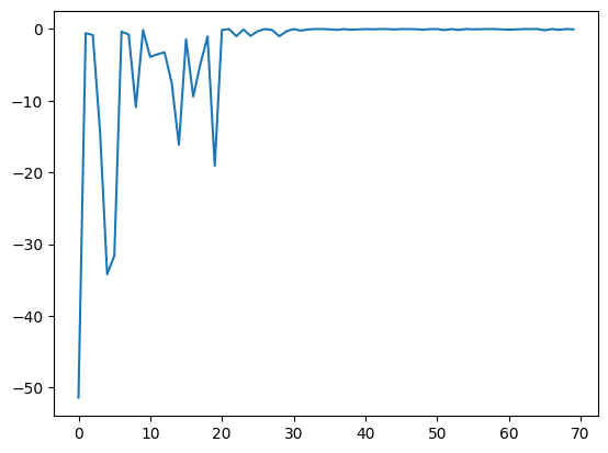
探索結果 res は history クラスのオブジェクト (physbo.search.discrete.results.history) として返されます。

以下より探索結果を参照します。

res.fx : simulator (目的関数) の評価値の履歴。
res.chosen_actions: simulator を評価したときの action ID (パラメータ) の履歴。
fbest, best_action= res.export_all_sequence_best_fx(): simulator を評価した全タイミングにおけるベスト値とその action ID (パラメータ)の履歴。
res.total_num_search: simulator のトータル評価数。

各ステップでの目的関数値と、ベスト値の推移をプロットしてみましょう。

res.fx, best_fx はそれぞれ res.total_num_search までの範囲を指定します。

[7]:

import matplotlib.pyplot as plt
%matplotlib inline

[8]:

plt.plot(res.fx[0:res.total_num_search])

[8]:

[<matplotlib.lines.Line2D at 0x148bbc5e0>]

../_images/notebook_tutorial_basic_15_1.png

[9]:

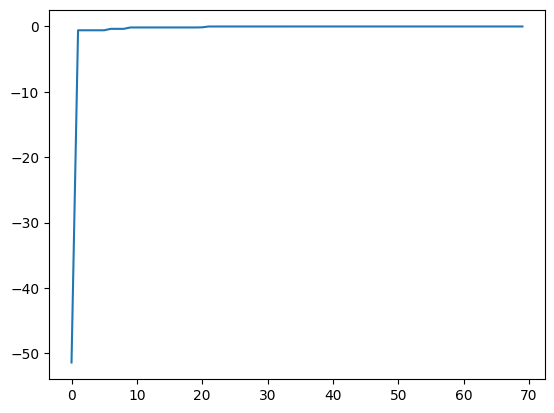
best_fx, best_action = res.export_all_sequence_best_fx()
plt.plot(best_fx)

[9]:

[<matplotlib.lines.Line2D at 0x148d05a90>]

../_images/notebook_tutorial_basic_16_1.png

結果のシリアライズ

探索結果は save メソッドにより外部ファイルに保存できます。

[10]:

res.save('search_result.npz')

[11]:

del res

保存した結果ファイルは以下のようにロードすることができます。

[12]:

res = physbo.search.discrete.History()
res.load('search_result.npz')

最後に、一番よいスコアを持つ候補は以下のようにして表示することができます。正しい解 x=-1に行き着いていることがわかります。

[13]:

print(X[int(best_action[-1])])

[-1.002]

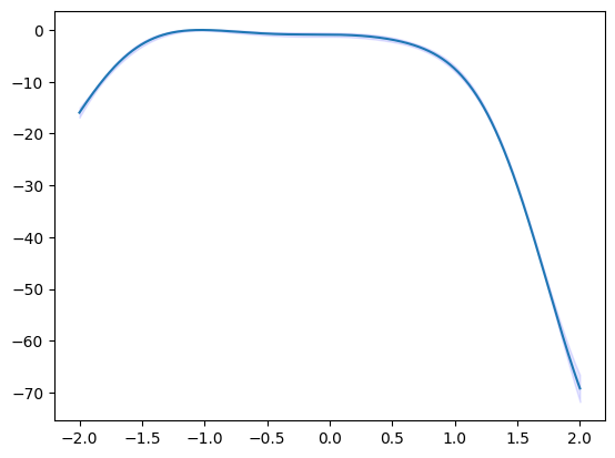
回帰

get_post_fmean, get_post_fcov メソッドでガウス過程（事後分布）の期待値と分散を計算可能です。

[14]:

mean = policy.get_post_fmean(X)
var = policy.get_post_fcov(X)
std = np.sqrt(var)

x = X[:,0]
fig, ax = plt.subplots()
ax.plot(x, mean)
ax.fill_between(x, (mean-std), (mean+std), color='b', alpha=.1)

[14]:

<matplotlib.collections.PolyCollection at 0x148d955b0>

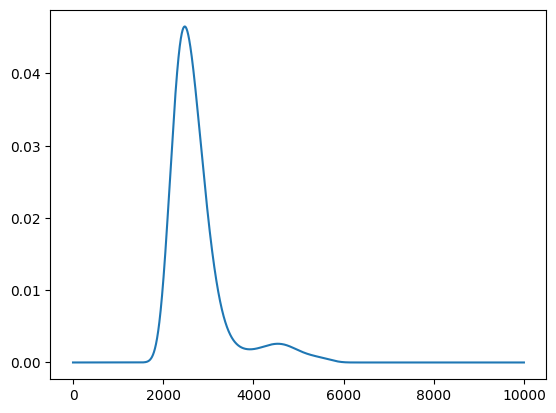
../_images/notebook_tutorial_basic_25_1.png

獲得関数

get_score メソッドで獲得関数を計算可能です。

[15]:

score = policy.get_score(mode="EI", xs=X)
plt.plot(score)

[15]:

[<matplotlib.lines.Line2D at 0x148e59e80>]

../_images/notebook_tutorial_basic_27_1.png

並列化

PHYSBO は全候補点に対する獲得関数の計算をMPI を用いて並列化出来ます。 MPI 並列には mpi4py を用います。

並列化を有効化するには、 policy のコンストラクタのキーワード引数 comm に MPI コミュニケータ、たとえば MPI.COMM_WORLD を渡してください。

[16]:

# from mpi4py import MPI
# policy = physbo.search.discrete.Policy(X=test_X, comm=MPI.COMM_WORLD)