4.4. DSQSS/DLA による正方格子上ハードコアボソン系の粒子数計算

このチュートリアルでは, 大きさ \(8\times8\) の正方格子上の, \(V/t=3, \beta t = 10\) というパラメータを持つハードコアボーズハバード模型について, 化学ポテンシャル \(\mu\) を \(-4.0\) から \(14.0\) まで動かして計算を行い, 粒子数密度の変化を計算します.

次に示すのは, 入力ファイルの生成と本計算を自動で行い, 粒子数密度の化学ポテンシャル依存性をファイルに書き出すスクリプトです(sample/dla/03_bosesquare/exec.py).

import sys
import os.path
import subprocess

bindir = sys.argv[1] if len(sys.argv) > 1 else ''

name = 'amzu'
mus = [-4.0, -2.0, 0.0, 2.0, 2.5, 3.0, 6.0, 9.0, 9.5, 10.0, 12.0, 14.0]

output = open('{}.dat'.format(name), 'w')

for i,mu in enumerate(mus):
    with open('std_{}.in'.format(i), 'w') as f:
        f.write('''
solver = DLA
model_type = boson
M = 1
J = 1
U = 0
V = 3
beta = 10.0
lattice_type = square
D = 2
L = 8,8
nset = 4
ntherm = 100
ndecor = 100
nmcs = 100
''')
        f.write('F = {}\n'.format(mu/4))
        f.write('algfile = algorithm_{}.xml\n'.format(i))
        f.write('outfile = res_{}.dat\n'.format(i))
    cmd = [os.path.join(bindir, 'dsqss_pre.py'),
           '-p', 'param_{}.in'.format(i),
           '-i', 'std_{}.in'.format(i)]
    subprocess.call(cmd)
    cmd = [os.path.join(bindir, 'dla_B'), 'param_{}.in'.format(i)]
    subprocess.call(cmd)
    with open('res_{}.dat'.format(i)) as f:
        for line in f:
            if not line.startswith('R'):
                continue
            words = line.split()
            if words[1] == name:
                output.write('{} {} {}\n'.format(mu, words[3], words[4]))

環境変数 $DSQSS_ROOT が設定されているならばそのまま実行できますが, そうでない場合は実行ファイルがインストールされているディレクトリを引数として渡します.

$ python exec.py $DSQSS_ROOT/bin

結果は amzu.dat に書き出されます(図 4.2). \(\mu=6\) 付近では密度プラトーが観測されます. ここでは近接サイト間の反発によりチェッカーボード固体相になっています.

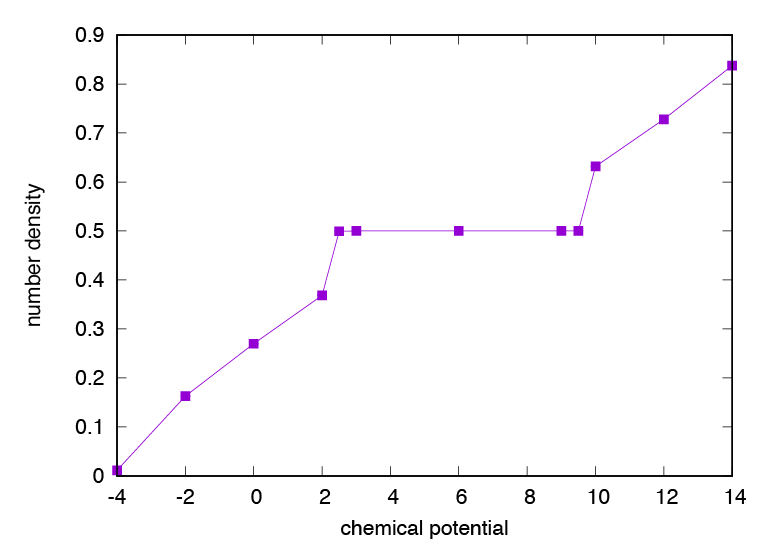
図 4.2 正方格子上のボースハバード模型における密度の化学ポテンシャル依存性.