Tensor train optimization (TTOpt)#
This tutorial explains how to minimize the Himmelblau function using the tensor-train optimization algorithm TTOpt. For an overview of the algorithm and a detailed description of the parameters, see Tensor Train Optimization ttopt.
Sample files#
Sample files are in sample/analytical/ttopt.
The directory contains the following:
input.tomlInput file for the main program
do.shScript to run this tutorial in one step
plot.pyScript that plots the search history on contours of the Himmelblau function
Input files#
Create the main input file input.toml.
For the full input specification, see the Input files chapter.
[base]
dimension = 2
output_dir = "output"

[solver]
name = "analytical"
function_name = "himmelblau"

[runner]
[runner.log]
interval = 20

[algorithm]
name = "ttopt"
seed = 12345

[algorithm.param]
max_list = [6.0, 6.0]
min_list = [-6.0, -6.0]

[algorithm.ttopt]
q_points = 20
max_f_eval = 1000
save_eval_history = true
The contents of [base], [solver], and [runner] sections are the same as those for the search by the Nelder-Mead method (minsearch).
The [algorithm] section selects the algorithm and its general settings.
nameis the algorithm name. This tutorial usesttopt.seedis the random seed.
The [algorithm.param] section sets the search region.
min_listandmax_listare lists of lower and upper bounds for each dimension.
The [algorithm.ttopt] section sets TTOpt-specific parameters.
q_pointsis the number of submodes (tensor legs) per dimension. If a single integer is given, it is applied to every dimension. Together withp_points(default 2 on each dimension), this sets the discretization; see Tensor Train Optimization ttopt.max_f_evalis the maximum number of function evaluations during the optimization.If
save_eval_historyistrue, evaluated points are appended tooutput/ttopt_eval_history.txt.
Other parameters (p_points, r_max, and so on) are omitted here and take their defaults; see the Input files chapter and Tensor Train Optimization ttopt.
Running the calculation#
Change to the tutorial directory (assuming you are at the root of the downloaded ODAT-SE package).
$ cd sample/analytical/ttopt
Run the main program. On a typical PC this finishes in a few seconds.
$ odatse input.toml | tee log.txt
You may also run everything at once with do.sh.
$ sh do.sh
When the run completes, a subdirectory for each rank appears under output (here output/0/). Standard output shows settings and progress. The optimization trace (function evaluation count and the best point and value so far) is written to output/ttopt_history.txt. Lines at the beginning starting with # describe the columns.
# $1: count
# $2: x_opt[0]
# $3: x_opt[1]
# $4: fx_opt
8 -2.731026392961877e+00 2.962437593877404e+00 1.247312995590882e+00
24 -2.731026392961877e+00 2.962437593877404e+00 1.247312995590882e+00
...
The first column is the number of function evaluations; the following columns are the coordinates of the best point so far and the objective f(x). Hyperparameters are listed in output/ttopt_hyperparameters.txt, and a short summary of the best solution is in output/res.txt, among others.
For example, res.txt is as follows:
fx = 7.17954154082022e-05
x1 = -2.805195622630713
x2 = 3.1299792575638374
Visualizing results#
Columns 2 and 3 of output/ttopt_history.txt correspond to the best x1 and x2 at each recorded step. The bundled plot.py overlays this trajectory on Himmelblau contours and saves a PDF.
$ python3 ./plot.py --xcol=1 --ycol=2 --format="-o" --output=output/res.pdf output/ttopt_history.txt
This creates output/res.pdf with the history of best-point updates from TTOpt. The iterate approaches a minimum already at an early stage.
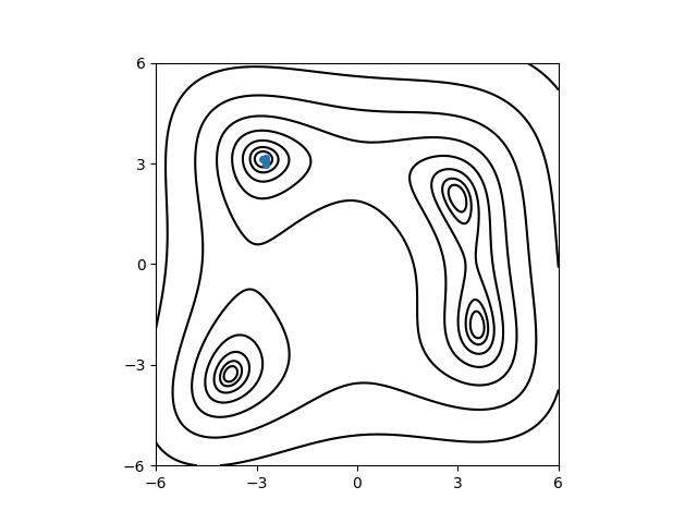
Fig. 6 Example of minimizing the Himmelblau function with TTOpt. Black lines are contours of the function; blue markers are the best-point history recorded in ttopt_history.txt.#