4.4. 三角格子・正方格子ハイゼンベルク模型の磁化過程

次に三角格子上で定義されたスピン\(S=1/2\)の量子ハイゼンベルク模型の磁化過程の計算を紹介します。 ハミルトニアンは以下のようになります:

\[\begin{aligned} H = J \sum_{\langle i,j \rangle}\sum_{\alpha}^{x,y,z} {S}_i^{\alpha} {S}_j^{\alpha} - h \sum_i S_i^z\end{aligned}\]

ここで\(\langle i, j\rangle\)は隣接サイトの組を表し、\(h\)は\(z\)方向にかけられた外部磁場の大きさを表します。 この模型の基底状態を計算し、ユニットセルの平均磁化 \(\langle S_z \rangle\equiv \frac{1}{N_u}\sum_i^{N_u} \langle S_i^z \rangle\)を磁場\(h\)の関数として求めてみましょう ( \(N_u\) はユニットセル内のサイト数)。

この計算を行うには、 sample/04_magnetization のディレクトリ内にある toml ファイル basic.toml と、pythonスクリプト tutorial_magnetization.py を利用します。 basic.toml ファイルには、模型の設定やパラメータなどが記述されています。

[parameter]
[parameter.general]
is_real = true

[parameter.simple_update]
num_step = 200
tau = 0.01

[parameter.full_update]
num_step = 0
tau = 0.01

[parameter.ctm]
iteration_max = 100
dimension = 10

[lattice]
type = "triangular lattice"
L = 3
W = 3
virtual_dim = 2
initial = "random"

[model]
type = "spin"
J = 1.0

lattice セクションで三角格子を指定しており、ユニットセルの大きさは\(3\times 3\)を指定しています。 ここでは計算を軽くするために、 simple update だけを行っており、虚時間の刻み幅\(\tau\)は\(\tau = 0.01\)としています。また簡単のため、\(J=1\)としています。この基本設定ファイルを用いて、 tutorial_magnetization.py では磁場を掃引したときの磁化を計算します。

import subprocess
from os.path import join
import numpy as np
import toml

MPI_cmd = ""  # e.g., "mpiexec -np 1"

num_h = 21
min_h = 0.0
max_h = 5.0
num_step_table = [100, 200, 500, 1000, 2000]

fmag = open("magnetization.dat", "w")
fene = open("energy.dat", "w")

for f in (fmag, fene):
    f.write("# $1: hz\n")
    for i, num_step in enumerate(num_step_table, 2):
        f.write(f"# ${i}: num_step={num_step}\n")
    f.write("\n")

for idx, h in enumerate(np.linspace(min_h, max_h, num=num_h)):
    print(f"Calculation Process: {idx+1}/{num_h}")
    inum = 0
    num_pre = 0
    fmag.write(f"{h} ")
    fene.write(f"{h} ")
    for num_step in num_step_table:
        ns = num_step - num_pre
        print(f"Steps: {num_step}")
        with open("basic.toml") as f:
            dict_toml = toml.load(f)

        output_dir = f"output_{idx}_{num_step}"

        dict_toml["parameter"]["general"]["output"] = output_dir
        dict_toml["parameter"]["general"]["tensor_save"] = "tensor_save"
        dict_toml["model"]["hz"] = float(h)
        dict_toml["parameter"]["simple_update"]["num_step"] = ns
        if inum > 0:
            dict_toml["parameter"]["general"]["tensor_load"] = "tensor_save"

        simple_toml = f"simple_{idx}_{num_step}.toml"
        std_toml = f"std_{idx}_{num_step}.toml"
        input_toml = f"input_{idx}_{num_step}.toml"

        with open(simple_toml, "w") as f:
            toml.dump(dict_toml, f)
        cmd = f"tenes_simple {simple_toml} -o {std_toml}"
        subprocess.call(cmd.split())

        cmd = f"tenes_std {std_toml} -o {input_toml}"
        subprocess.call(cmd.split())

        cmd = f"{MPI_cmd} tenes {input_toml}"
        subprocess.call(cmd.split())

        ene = 0.0
        mag_sz = 0.0
        with open(join(output_dir, "density.dat")) as f:
            for line in f:
                name, vals = line.split("=")
                if name.strip() == "Energy":
                    re, im = vals.split()
                    ene += float(re)
                elif name.strip() == "Sz":
                    re, im = vals.split()
                    mag_sz += float(re)
        fene.write(f"{ene} ")
        fmag.write(f"{mag_sz} ")
        inum = inum + 1
        num_pre = num_step
    fene.write("\n")
    fmag.write("\n")
fene.close()
fmag.close()

このスクリプトでは、磁場\(h\)を0から5まで0.25刻みで変化させ、基底状態のエネルギーと\(\langle S_z \rangle\)を計算して、 energy.dat および magnetization.dat に出力します。 simple update の時間ステップ数を\(100\), \(200\), \(500\), \(1000\), \(2000\)と変化させたときの様子を見るために、各磁場でステップ数を変えた計算も行っています。 計算量を減らすために、少ないステップ数で得られた波動関数の情報を tensor_save に保存し、それをより多いステップ数の計算の初期状態としてとっています。例えば、最初に時間ステップ数を100とした計算を行って結果を出力したあと、ステップ数100の計算終了時の波動関数からさらにステップ数100の計算を行って、結果的にステップ数200の計算結果を得ます。

実際に実行してみましょう。あらかじめ tenes などにパスを通した上で

python tutorial_magnetization.py

により計算を実行します。ノートPC(シングルプロセッサ)では数時間程度の計算量となります。 計算が終了したら、gnuplotを起動し、

load 'plot.gp'

とすれば、図 4.5 の右図のような磁化カーブが得られます。同様に

load 'plot_ene.gp'

とすれば、図 4.5 の左図のような基底エネルギーのグラフが得られます。

十分なステップ数(例えばステップ数2000)の計算結果からわかるように、磁化過程には飽和磁化\(\langle S_z \rangle=0.5\)の\(1/3\)の磁化のところで、プラトー構造が生じます。 このプラトー上では、3つの格子上のスピンが\(\uparrow\), \(\uparrow\), \(\downarrow\)と磁化した周期構造を形成し、スピンギャップが生じています。このプラトー構造は三角格子特有のものです。 実際に計算精度がでているかどうかをみるには、エネルギーのステップ依存性が参考になります。 理想的にはステップ数を増やすほど基底エネルギーが下がるはずですが、一部の磁場領域では逆に基底エネルギーが増加します。これは計算精度があまりでていない兆候です。 ボンド次元を増やすなどして、より計算精度を高める必要があると推測されます。

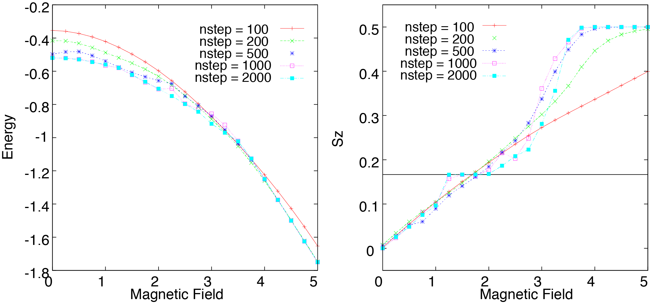
図 4.5 三角格子量子ハイゼンベルク模型のエネルギー(左図)と磁化過程(右図)

では正方格子でも同じことをやってみましょう。 sample/04_magnetization のディレクトリ中にある toml ファイル basic_square.toml と、pythonスクリプト tutorial_magnetization_square.py を利用します。 basic_square.toml は、 lattice セクションが以下のように変更されているほかは basic.toml と同じ内容です。

[lattice]
type = "square lattice"
L = 2
W = 2

実際に計算を行うには、

python tutorial_magnetization_square.py

とします。計算が終了したら、gnuplotを起動し、

load 'plot_square.gp'

とすれば、 図 4.6 の右図のような磁化カーブが得られます。同様に

load 'plot_square_ene.gp'

とすれば、図 4.6 の左図のような基底エネルギーのグラフが得られます。

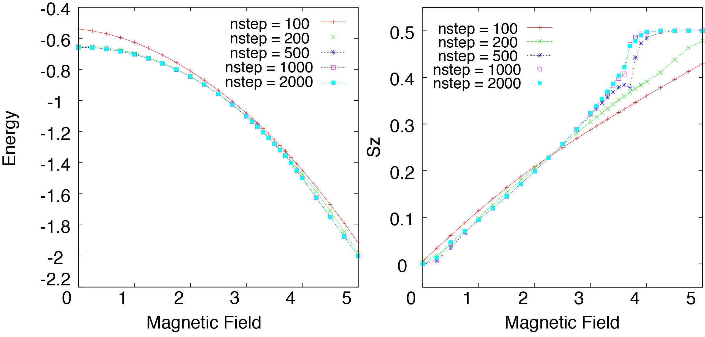
図 4.6 正方格子量子ハイゼンベルク模型のエネルギー(左図)と磁化過程(右図)

ステップ数2000でほぼ収束しており、三角格子ハイゼンベルク模型と異なり、プラトー構造は現れないことがわかります。 エネルギーは概ね、ステップ数を増加させると減少するため、ある程度計算精度がでていると推測されます。