4.1. 横磁場イジング模型

ここでは正方格子上の横磁場イジング模型に対して、横磁場を変化させた場合の計算例について紹介します。 ハミルトニアンは

\[\begin{aligned} H = J^z \sum_{\langle i,j \rangle} {S}_i^{z} {S}_j^{z} - h^x \sum_i S_i^x \end{aligned}\]

です。 大きさ1/2のスピン演算子を用いて定義しており、パウリ演算子を直接用いたモデルと係数が異なることに注意してください。 入力ファイルの変数 hx を用いることで横磁場 \(h^x\) の大きさを調整することが可能です。例えば、横磁場が0の場合には、

[parameter]
[parameter.general]
is_real = true  # Limit tensor elements in real (not complex)

[parameter.simple_update]
num_step = 1000 # Number of steps in simple update
tau = 0.01      # Imaginary time slice

[parameter.full_update]
num_step = 0    # Number of steps in full update
tau = 0.01      # Imaginary time slice

[parameter.ctm]
meanfield_env = false # Use meanfield environment to contract iTNS
iteration_max = 10    # Maximum number of iterations in CTMRG
dimension = 10        # Bond dimension of corner transfer matrix

[lattice]
type = "square lattice" # Type of lattice
L = 2                   # X length of unit cell
W = 2                   # Y length of unit cell
virtual_dim = 2         # Bond dimension of bulk tensors
initial = "ferro"       # Initial condition

[model]
type = "spin" # Type of model
Jz = -1.0     # Jz SzSz
Jx = 0.0      # Jx SxSx
Jy = 0.0      # Jy SySy
hx = 0.0      # hx Sx

とします(Jz = -1.0 なので、 hx=0 では強磁性状態になります)。入力ファイルを simple.toml とした場合、

$ tenes_simple simple.toml
$ tenes_std std.toml
$ tenes input.toml

を実行することで計算が開始されます。 （あらかじめ TeNeS をインストールしたのち、環境変数 PATH を適切に設定してください。） 計算を実行すると、

Number of Processes: 1
Number of Threads / Process: 1
Tensor type: real
Start simple update
10% [100/1000] done
20% [200/1000] done
30% [300/1000] done
40% [400/1000] done
50% [500/1000] done
60% [600/1000] done
70% [700/1000] done
80% [800/1000] done
90% [900/1000] done
100% [1000/1000] done
Start calculating observables
Start updating environment
Start calculating onesite operators
Save onesite observables to output_0/onesite_obs.dat
Start calculating twosite operators
Save twosite observables to output_0/twosite_obs.dat
Save observable densities to output_0/density.dat
Save elapsed times to output_0/time.dat

Onesite observables per site:
Sz          = 0.5 0
Sx          = -1.28526262482e-13 0
Twosite observables per site:
hamiltonian = -0.5 0
SzSz        = 0.5 0
SxSx        = -1.7374919982e-18 0
SySy        = 1.73749202733e-18 0
Wall times [sec.]:
simple update = 3.545813509
full update   = 0
environmnent  = 0.123170523
observable    = 0.048149856

Done.

のように計算が実行されます。 最初に並列化の情報およびテンソルの実虚が表示されます。 次に計算プロセスの実行状況が表示されます。 計算終了後、 1サイト演算子 Sz, Sx およびハミルトニアン hamiltonian , 最近接相関 SzSz, SxSx, SySy のサイトあたりの期待値が出力されます。 最後にフェーズごとの計算時間が出力されます(単位は秒)。 計算終了後は output ディレクトリに density.dat, parameters.dat, time.dat, onesite_obs.dat, twosite_obs.dat がそれぞれ出力されます。各出力ファイルの詳細は、 出力ファイル をご覧ください。 例えば <Sz> の値は、 onesite_obs.dat から読み取ることが可能です。 hx をパラメータとして0.2刻みで0-3.0まで振ったときの結果を下図に表示します。

なお、サンプルスクリプトの例として、 sample/01_transverse_field_ising フォルダ内に tutorial_example.py , tutorial_read.py があります。

• tutorial_example.py の中身

import subprocess

import numpy as np
import toml

MPI_cmd = ""  # e.g., "mpiexec -np 1"

num_hx = 16
min_hx = 0.0
max_hx = 3.0

total = 0
for idx, hx in enumerate(np.linspace(min_hx, max_hx, num=num_hx)):
    print(f"Calculation Process: {idx+1}/{num_hx}")
    with open("simple.toml") as f:
        dict_toml = toml.load(f)
    dict_toml["parameter"]["general"]["output"] = f"output_{idx}"
    dict_toml["model"]["hx"] = float(hx)

    simple_toml = f"simple_{idx}.toml"
    std_toml = f"std_{idx}.toml"
    input_toml = f"input_{idx}.toml"

    with open(simple_toml, "w") as f:
        toml.dump(dict_toml, f)
    cmd = f"tenes_simple {simple_toml} -o {std_toml}"
    subprocess.call(cmd.split())

    cmd = f"tenes_std {std_toml} -o {input_toml}"
    subprocess.call(cmd.split())

    cmd = f"{MPI_cmd} tenes {input_toml}"
    subprocess.call(cmd.split())

• tutorial_read.py の中身

from os.path import join

import toml

num_hx = 16

print("# $1: h")
print("# $2: ene")
print("# $3: sz")
print("# $4: sx")
print()

for idx in range(num_hx):
    try:
        with open(f"simple_{idx}.toml") as f:
            dict_toml = toml.load(f)
        hx = dict_toml["model"]["hx"]
        ene = 0.0
        mag_sz = 0.0
        mag_sx = 0.0
        with open(join(f"output_{idx}", "density.dat")) as f:
            for line in f:
                words = line.split()
                if words[0] == "Energy":
                    ene = words[2]
                elif words[0] == "Sz":
                    mag_sz = words[2]
                elif words[0] == "Sx":
                    mag_sx = words[2]
        print(f"{hx} {ene} {mag_sz} {mag_sx}")
    except:
        continue

あらかじめ tenes などにパスを通した上で

$ python tutorial_example.py

として実行できます(MacBook2017, 1.4 GHz Intel Core i7で数分程度で計算が全て終了します)。 得られた結果は

$ python tutorial_read.py

とすることで集計でき、 hx, エネルギー、 <Sz> 、 <Sx> が出力されます。

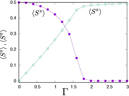
図 4.1 <Sz> , <Sx> の hx 依存性

図 4.1 から hx が大きくなるにつれ、 <Sz> が 0.5 から徐々に小さくなり最終的には0になる一方、 <Sx> は 0 から大きくなり最終的には 0.5 になることが分かります。